Tfrecords Guide
A post showing how to convert your dataset to .tfrecords file and later on use it as a part of a computational graph.
Introduction
In this post we will cover how to convert a dataset into .tfrecord file. Binary files are sometimes easier to use, because you don’t have to specify different directories for images and groundtruth annotations. While storing your data in binary file, you have your data in one block of memory, compared to storing each image and annotation separately. Openning a file is a considerably time-consuming operation especially if you use hdd and not ssd, because it involves moving the disk reader head and that takes quite some time. Overall, by using binary files you make it easier to distribute and make the data better aligned for efficient reading.
The post consists of tree parts: in the first part, we demonstrate how you can get raw data bytes of any image using numpy which is in some sense similar to what you do when converting your dataset to binary format. Second part shows how to convert a dataset to tfrecord file without defining a computational graph and only by employing some built-in tensorflow functions. Third part explains how to define a model for reading your data from created binary file and batch it in a random manner, which is necessary during training.
The blog post is created using jupyter notebook. After each chunk of a code you can see the result of its evaluation. You can also get the notebook file from here.
Getting raw data bytes in numpy
Here we demonstrate how you can get raw data bytes of an image (any ndarray) and how to restore the image back. We point out that during this operation the information about the dimensions of the image is lost and we have to use it to recover the original image. This is one of the reasons why we will have to store the raw image representation along with the dimensions of the original image.
In the following examples, we convert the image into the raw representation, restore it and make sure that the original image and the restored one are the same.
%matplotlib inline
import numpy as np
import skimage.io as io
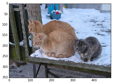
cat_img = io.imread('cat.jpg')
io.imshow(cat_img)
<matplotlib.image.AxesImage at 0x7f8dc8cb3310>
# Let's convert the picture into string representation
# using the ndarray.tostring() function
cat_string = cat_img.tostring()

# Now let's convert the string back to the image
# Important: the dtype should be specified
# otherwise the reconstruction will be errorness
# Reconstruction is 1d, so we need sizes of image
# to fully reconstruct it.
reconstructed_cat_1d = np.fromstring(cat_string, dtype=np.uint8)

# Here we reshape the 1d representation
# This is the why we need to store the sizes of image
# along with its serialized representation.
reconstructed_cat_img = reconstructed_cat_1d.reshape(cat_img.shape)

# Let's check if we got everything right and compare
# reconstructed array to the original one.
np.allclose(cat_img, reconstructed_cat_img)
True
Creating a .tfrecord file and reading it without defining a graph
Here we show how to write a small dataset (three images/annotations from PASCAL VOC) to .tfrrecord file and read it without defining a computational graph.
We also make sure that images that we read back from .tfrecord file are equal to the original images. Pay attention that we also write the sizes of the images along with the image in the raw format. We showed an example on why we need to also store the size in the previous section.
# Get some image/annotation pairs for example
filename_pairs = [
('/home/dpakhom1/tf_projects/segmentation/VOCdevkit/VOCdevkit/VOC2012/JPEGImages/2007_000032.jpg',
'/home/dpakhom1/tf_projects/segmentation/VOCdevkit/VOCdevkit/VOC2012/SegmentationClass/2007_000032.png'),
('/home/dpakhom1/tf_projects/segmentation/VOCdevkit/VOCdevkit/VOC2012/JPEGImages/2007_000039.jpg',
'/home/dpakhom1/tf_projects/segmentation/VOCdevkit/VOCdevkit/VOC2012/SegmentationClass/2007_000039.png'),
('/home/dpakhom1/tf_projects/segmentation/VOCdevkit/VOCdevkit/VOC2012/JPEGImages/2007_000063.jpg',
'/home/dpakhom1/tf_projects/segmentation/VOCdevkit/VOCdevkit/VOC2012/SegmentationClass/2007_000063.png')
                 ]
%matplotlib inline

# Important: We are using PIL to read .png files later.
# This was done on purpose to read indexed png files
# in a special way -- only indexes and not map the indexes
# to actual rgb values. This is specific to PASCAL VOC
# dataset data. If you don't want thit type of behaviour
# consider using skimage.io.imread()
from PIL import Image
import numpy as np
import skimage.io as io
import tensorflow as tf


def _bytes_feature(value):
    return tf.train.Feature(bytes_list=tf.train.BytesList(value=[value]))

def _int64_feature(value):
    return tf.train.Feature(int64_list=tf.train.Int64List(value=[value]))

tfrecords_filename = 'pascal_voc_segmentation.tfrecords'

writer = tf.python_io.TFRecordWriter(tfrecords_filename)

# Let's collect the real images to later on compare
# to the reconstructed ones
original_images = []

for img_path, annotation_path in filename_pairs:

    img = np.array(Image.open(img_path))
    annotation = np.array(Image.open(annotation_path))

    # The reason to store image sizes was demonstrated
    # in the previous example -- we have to know sizes
    # of images to later read raw serialized string,
    # convert to 1d array and convert to respective
    # shape that image used to have.
    height = img.shape[0]
    width = img.shape[1]

    # Put in the original images into array
    # Just for future check for correctness
    original_images.append((img, annotation))

    img_raw = img.tostring()
    annotation_raw = annotation.tostring()

    example = tf.train.Example(features=tf.train.Features(feature={
        'height': _int64_feature(height),
        'width': _int64_feature(width),
        'image_raw': _bytes_feature(img_raw),
        'mask_raw': _bytes_feature(annotation_raw)}))

    writer.write(example.SerializeToString())

writer.close()
reconstructed_images = []

record_iterator = tf.python_io.tf_record_iterator(path=tfrecords_filename)

for string_record in record_iterator:

    example = tf.train.Example()
    example.ParseFromString(string_record)

    height = int(example.features.feature['height']
                                 .int64_list
                                 .value[0])

    width = int(example.features.feature['width']
                                .int64_list
                                .value[0])

    img_string = (example.features.feature['image_raw']
                                  .bytes_list
                                  .value[0])

    annotation_string = (example.features.feature['mask_raw']
                                .bytes_list
                                .value[0])

    img_1d = np.fromstring(img_string, dtype=np.uint8)
    reconstructed_img = img_1d.reshape((height, width, -1))

    annotation_1d = np.fromstring(annotation_string, dtype=np.uint8)

    # Annotations don't have depth (3rd dimension)
    reconstructed_annotation = annotation_1d.reshape((height, width))

    reconstructed_images.append((reconstructed_img, reconstructed_annotation))
# Let's check if the reconstructed images match
# the original images

for original_pair, reconstructed_pair in zip(original_images, reconstructed_images):

    img_pair_to_compare, annotation_pair_to_compare = zip(original_pair,
                                                          reconstructed_pair)
    print(np.allclose(*img_pair_to_compare))
    print(np.allclose(*annotation_pair_to_compare))
True
True
True
True
True
True
Defining the graph to read and batch images from .tfrecords
Here we define a graph to read and batch images from the file that we have created previously. It is very important to randomly shuffle images during training and depending on the application we have to use different batch size.
It is very important to point out that if we use batching – we have to define the sizes of images beforehand. This may sound like a limitation, but actually in the Image Classification and Image Segmentation fields the training is performed on the images of the same size.
The code provided here is partially based on this official example and code from this stackoverflow question. Also if you want to know how you can control the batching according to your need read these docs .
%matplotlib inline

import tensorflow as tf
import skimage.io as io

IMAGE_HEIGHT = 384
IMAGE_WIDTH = 384

tfrecords_filename = 'pascal_voc_segmentation.tfrecords'

def read_and_decode(filename_queue):

    reader = tf.TFRecordReader()

    _, serialized_example = reader.read(filename_queue)

    features = tf.parse_single_example(
      serialized_example,
      # Defaults are not specified since both keys are required.
      features={
        'height': tf.FixedLenFeature([], tf.int64),
        'width': tf.FixedLenFeature([], tf.int64),
        'image_raw': tf.FixedLenFeature([], tf.string),
        'mask_raw': tf.FixedLenFeature([], tf.string)
        })

    # Convert from a scalar string tensor (whose single string has
    # length mnist.IMAGE_PIXELS) to a uint8 tensor with shape
    # [mnist.IMAGE_PIXELS].
    image = tf.decode_raw(features['image_raw'], tf.uint8)
    annotation = tf.decode_raw(features['mask_raw'], tf.uint8)

    height = tf.cast(features['height'], tf.int32)
    width = tf.cast(features['width'], tf.int32)

    image_shape = tf.pack([height, width, 3])
    annotation_shape = tf.pack([height, width, 1])

    image = tf.reshape(image, image_shape)
    annotation = tf.reshape(annotation, annotation_shape)

    image_size_const = tf.constant((IMAGE_HEIGHT, IMAGE_WIDTH, 3), dtype=tf.int32)
    annotation_size_const = tf.constant((IMAGE_HEIGHT, IMAGE_WIDTH, 1), dtype=tf.int32)

    # Random transformations can be put here: right before you crop images
    # to predefined size. To get more information look at the stackoverflow
    # question linked above.

    resized_image = tf.image.resize_image_with_crop_or_pad(image=image,
                                           target_height=IMAGE_HEIGHT,
                                           target_width=IMAGE_WIDTH)

    resized_annotation = tf.image.resize_image_with_crop_or_pad(image=annotation,
                                           target_height=IMAGE_HEIGHT,
                                           target_width=IMAGE_WIDTH)


    images, annotations = tf.train.shuffle_batch( [resized_image, resized_annotation],
                                                 batch_size=2,
                                                 capacity=30,
                                                 num_threads=2,
                                                 min_after_dequeue=10)

    return images, annotations
filename_queue = tf.train.string_input_producer(
[tfrecords_filename], num_epochs=10)
# Even when reading in multiple threads, share the filename
# queue.
image, annotation = read_and_decode(filename_queue)
# The op for initializing the variables.
init_op = tf.group(tf.global_variables_initializer(),
tf.local_variables_initializer())
with tf.Session() as sess:
sess.run(init_op)
coord = tf.train.Coordinator()
threads = tf.train.start_queue_runners(coord=coord)
# Let's read off 3 batches just for example
for i in xrange(3):
img, anno = sess.run([image, annotation])
print(img[0, :, :, :].shape)
print('current batch')
# We selected the batch size of two
# So we should get two image pairs in each batch
# Let's make sure it is random
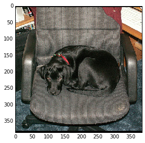
io.imshow(img[0, :, :, :])
io.show()
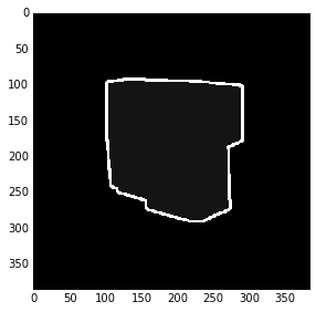
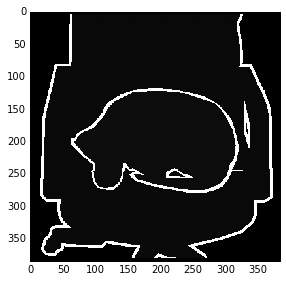
io.imshow(anno[0, :, :, 0])
io.show()
io.imshow(img[1, :, :, :])
io.show()
io.imshow(anno[1, :, :, 0])
io.show()
coord.request_stop()
coord.join(threads)
(384, 384, 3)
current batch
(384, 384, 3)
current batch


(384, 384, 3)
current batch


Conclusion and Discussion
In this post we covered how to convert a dataset into .tfrecord format, made sure that we didn’t corrupt the data and saw how to define a graph to read and batch files from the created file.