An introduction post about my project where I describe the chosen Face Detection algorithm, explain why it was chosen and briefly go over all the stages of it.

---

Algorithm choice

Usually, when it goes to the Face Recognition task, the most important criteria are:

1. Good False Positive and False Negatives ratio (ratio of amount of objects classified as faces to amount of faces classified as non-faces).
2. Speed. Possibility of a real-time performance.
3. Affordable algorithm training time.

The algorithm that satisfies all these criteria is Viola-Jones Face Detection algorithm. The training stage can take quite a while but characteristics of the algorithm are very good. The problem with this algorithm is that it is patented and can’t be safely used.

There are two possible ways to solve this problem:

1. Find a way to avoid the patent in Viola-Jones Face Detection algorithm.
2. Implement another patent-free Face Detection Algorithm.

I investigated both ways and decided upon implementing another algorithm. I will give detailed description of my investigation in the following two sections.

Approach one: avoid patent

When I was reading a beautiful description of Viola-Jones Face Detection algorithm, I found out how OpenCv solved the problem with the patent. I will cite the above description:

Interestingly enough, therein laid a solution to a untold problem: Viola and Jones had patented their algorithm. So in order to use it commercially, you would have to license if from the authors, possibly paying a fee. As a way to extend the detector, Dr. Rainer Lienhart, the original implementer of the OpenCV Haar feature detector, proposed adding two new types of features and transforming each weak learner into a tree. This later trick, besides helping in the classification, was also sufficient to get out of the patent protection of the original method.

So, it is not a problem to avoid the patent by following the way of OpenCv, but I decided to investigate the second option.

Approach two: different algorithm

While searching for alternatives, I found a paper named “Face Detection Based on Multi-Block LBP Representation” that describes an algorithm that is similar to Viola-Jones Face Detection algorithm, but uses different features and different learning algorithm and is not patented. In the paper, authors state that the algorithm has better results than Viola-Jones Face Detection algorithm and can be trained in less time. Moreover, I found out that this algorithm is also implemented by OpenCv.

The fact that the algorithm can be trained much faster is a very crucial, because one stage of developing a Face Detection algorithm is hyperparameter optimization (tuning parameters of the algorithm to make it work better). If we spend less time on training, we can search for best parameters more thoroughly.

These facts all together made me choose this algorithm.

Algorithm description

The chosen algorithm consists of the following parts:

1. Features: Multiblock Local Binary Patterns for image patch description.
2. Training: Gentle Adaboost algorithm for feature selection(choosing the most discriminative features).
3. Cascade: early rejection of “obvious” non-faces. The same as in Viola-Jones algorithm.

Multiblock Local Binary Patterns

The algorithm uses Multiblock Local Binary Patterns, an improvement of Local Binary Patterns that can be computed at multiple scales and is very good suited for usage with integral images.

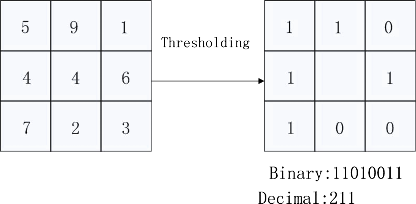
The basic idea behind the LBP is that they encode each pixel using its intensity value and intensity values of surrounding pixels. Depending on what pixels out of surrounding have greater or smaller intensity value, the pixel gets a specific 8-bit binary code that is later translated into number:

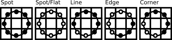
Also, the intensity values are taken from a circle surrounding selected pixel. The points are sampled evenly and their values has to be interpolated. Each pattern represents a particular structure:

When it comes to Multiblock Local Binary Patterns we:

1. Take average intensity values of surrounding blocks.
2. Don’t use interpolation.

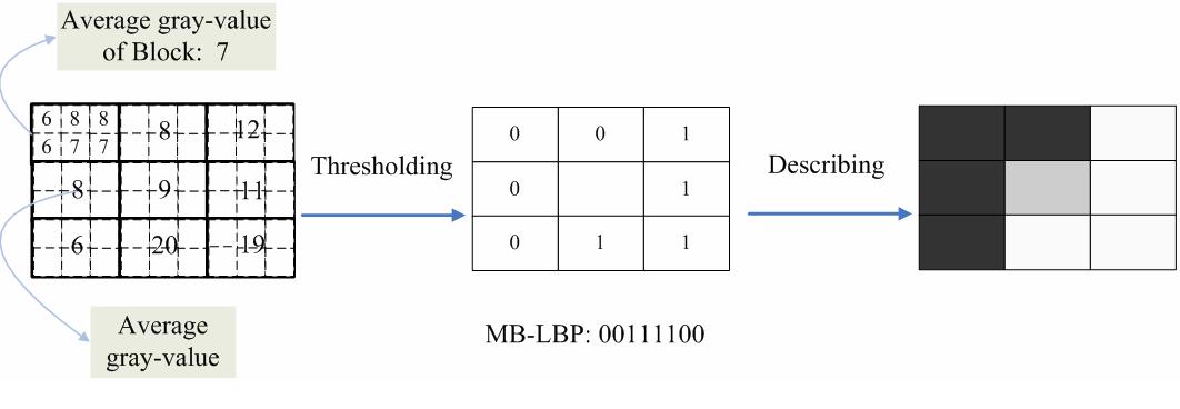
This structure can be scaled and, therefore, can capture patterns on different scale levels. Moreover, if we use integral image representation, these patterns can be computed in a constant time, not depending on the scale of a pattern.

Scikit-image already has LBP implementation and integral image representation. This fact will make the development much easier.

Gentle Adaboost training algorithm

The next stage of our algorithm is to find out what patterns out of all possible are the best in discriminating faces from non-faces.

In case of haar features, that are used by Viola-Jones algorithm, the most useful features are:

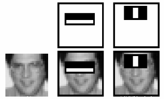
As you can see, the training algorithm found out that on images of faces the region of nose is usually brighter than region of eyes (right bottom picture).

We will do the same but for Multi-block binary patterns: find the features that help us find faces with better accuracy.

The usual problem with the training stage is that we have to scan through a lot of different possible features and check each time how good a particular feature works on the whole training corpus.

In case of Viola-Jones algorithm, given a sub-window size of $20\times20$, there are totally $45891$ possible features. This is the reason why it takes so much for the algorithm to train. Also, this is why the algorithm of Viola and Jones uses more aggressive training algorithm called Adaboost to decrease the amount “probably” good features as much as possible on each training step.

MB-LBP has totally $2049$ features in the same sub-window region. It reduces the training time drastically and enables to use more precise training algorithms. In the selected paper the Gentle Adaboost training algorithm is used. The difference from the Adaboost is that it has better generalization performance. This means that results showed by Adaboost can be good on training set, but when it comes to a real world data, the performance degrades. I will cite Wikipedia on that:

Empirical observations about the good performance of GentleBoost appear to back up Schapire and Singer’s remark that allowing excessively large values of $\alpha$ can lead to poor generalization performance.

To briefely describe how the training algorithms of the boosting approach work: we take the whole training set and find a feature(like in the case of nose region) that has the best discriminative power by itself. In other words we have a “rule of thumb” that the brighter region of nose is a good sign of a face in an image. In literature this “rule of thumb” is called a weak classifier:

Weak classifiers (or weak learners) are classifiers which perform only slightly better than a random classifier. These are thus classifiers which have some clue on how to predict the right labels, but not as much as strong classifiers have like , e.g., Naive Bayes, Neural Networks or SVM.

After that, we save our weak classifier and give less weights to the training images that it classified correctly and more weight to the misclassified ones. That way, next classifiers focus on the hard examples that were were not classified correctly by all the previous weak classifiers. This process is repeated multiple times until the desired accuracy is not achieved.

When implementing this algorithm, I will use Scikit-learn machine learning library. The library doesn’t have the Gentle Adaboost implemented, but according to the following issue it can be easily implemented by changing the cost function. This may require a writing a small pull request to the mentioned library.

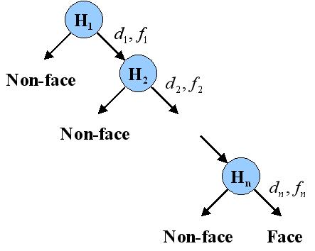
Cascade of classifiers

This part of the selected algorithm is the same as in the Viola-Jones algorithm. The main idea behind it is that some examples, that we want to classify, are easy and we don’t have to evaluate all of our leaned weak classifiers. For example, it’s easy for the algorithm to understand that image of a pen is not a face. But some examples are hard for classifier:

This is why we use cascade of classifiers: to reject non-faces early on and spend more time only on complicated examples.

This part can be probably also implemented with the help of Scikit-learn, but I need to investigate it further.

Training data set

Authors of the selected paper, used faces images from multiple sources and they don’t specify which databases they used. It is not a problem because there are multiple available databases of faces.

Another thing that we will have to do is to generate new samples out of available faces images by using random transformations like mirroring, small random shifting, rotation and scaling. By the described augmenting of our data set, we will make the algorithm more robust.

Community bonding period

During community bonding period I inspected the OpenCv library and tried to understand it much better. This is important because I plan to read OpenCv’s implementation of the selected paper in order to learn from it and to avoid some mistakes in the future.

Moreover, I read about Scikit-image packages that I will probably have to use. These are packages related to transformations, integral images, local binary patterns and related.

I also interacted with the community and I have to say that from the very beginning (from my first pull request) I feel that everybody in it is very responsible and tries to help as much as possible. And I am sure that I will learn a lot among them during this Summer.

I also want to thank Vignesh and Stefan. They helped me make my way from the idea of this project to the current state.