Here I will go into the details of implementing the training part of face detection algorithm and the difficulties that I faced.

---

Overall description of the training process.

The training consists of two logical parts:

1. Training the classifier using Gentle Adaboost.
2. Creating the Attentional cascade using trained classifiers.

The Gentle Adaboost part was implemented with the help of the original MBLBP paper but with a little difference in the tree implementation as in OpenCV, which was very hard to do because there are very little web resources or papers available online with description on how the algorithm works. And I had to read the source code. I will go into details about it in the respective section.

The cascade creation part was implemented using the Viola and Jones paper.

One more problem that I have faced during implementation was that I had to write everything using Cython without Python calls, because the training code should be very efficient, otherwise it will take to long to train a classifier for user. I had to do everything without using any numpy matrix operations. Also that fact that I was working with raw arrays made the debugging really hard.

I wasn’t able to finish the training part by the deadline of GSOC and had to work a little bit more which didn’t count towards GSOC but still I wanted to finish this part.

Gentle Adaboost.

The Gentle Adaboost works by training classifiers based on the training set and weights which describe the importance of a particular training example. In our case we have faces and non-faces. When it starts, it trains a decision tree with equal weights for each example. After the training, some examples are misclassified. Therefore, we put more weight on the examples that were misclassified and less weight on the examples that were correctly classified and train another decision tree using new weights. Then we repeat the same process and at the end we have a strong classifier that combines outputs of multiple weak ones (decision trees in our case). This algorithm is used to create strong classifiers for each stage of our cascade.

The one big problem that I faced was that the decision trees that are used in the the original MBLBP paper and the decision trees that are used by OpenCV are different. The original paper uses a regression decision tree with 256 branches and OpenCV uses a binary decision tree.

Because we followed the OpenCV APi from the very beginning I had to figure out how to train binary tree for our case. The problem seems easy, but it’s not.

As we use Multi-block Binary Patterns, that means that the features (patterns themselves) are categorical variables. For example, numbers are not categorical variables and can be easily ordered and compared to each other. So, in case of numbers if we have $n$ values we have to check $n-1$ possible split values. When we deal with categorical variables like colors (red, blue, black and so on) and Multi-block Binary Patterns it means that we can’t compare or order them, so in order to find a best split if we have $n$ values we have to try $2^{n-1}$ possibles splits. For example, in case of colors (red, blue, black, green) one possible split will be red and blue go to the right branch and others go to the right one. In case of Multi-block Binary Patterns we have $256$ values and it means that we have to check $2^{255}$ possible splits which is not feasible.

While reading the OpenCV documentation about decision trees I have found that there is a special algorithm for this particular case:

In case of regression and 2-class classification the optimal split can be found efficiently without employing clustering, thus the parameter is not used in these cases.

So, as we can see OpenCV uses clustering to solve this problem but in our case it doesn’t use it and instead just mentions that this task can be solved efficiently without clustering.

The only citation that the OpenCV documentation has is:

Breiman, L., Friedman, J. Olshen, R. and Stone, C. (1984), Classification and Regression Trees, Wadsworth.

Which I wasn’t able to find fully and it was only partially included in some lectures where the part mentioning the special algorithm wasn’t available.

After this I started to read the source code of OpenCV related to this problem. I found a function that is responsible for this algorithm but it was really hard to understand what is happening there because the code doesn’t have any citations of the original algorithm or its description.

Finally after spending a lot of time on this I found a one sentence description of that algorithm in the matlab’s description of tree module:

The tree can order the categories by mean response (for regression) or class probability for one of the classes (for classification). Then, the optimal split is one of the L – 1 splits for the ordered list. When K = 2, fitctree always uses an exact search.

So the main idea of the algorithm is to sort each of our categorical variable based on its mean response from training data. In this case we can compare them based on this values and treat them like numbers, reducing the complexity from exponential case to linear.

It was really strange that I found no description of this algorithm online and only this sentence that I found just by chance. It may be the case that this particular case is really rare in real world and nobody teaches it.

One more observation that I had is that by using the original tree from the paper we have a faster training process and a better one but a little bit slower evaluation part. I think in the future after more experiments we can also support the training that uses the original tree from the paper. By now we have the binary decision tree like in the OpenCV.

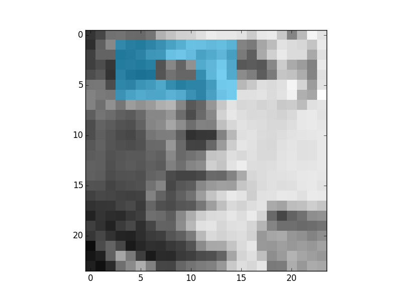
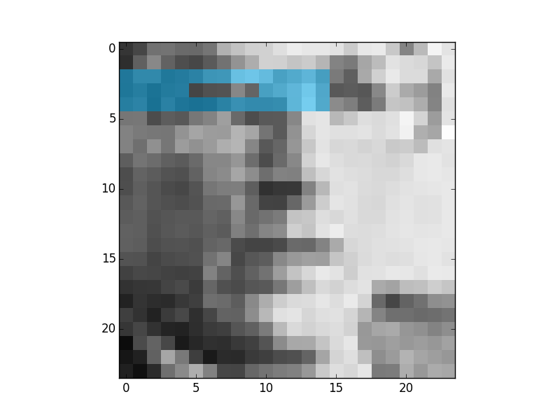
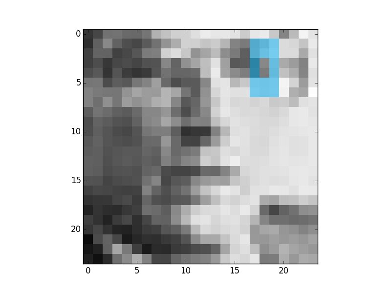
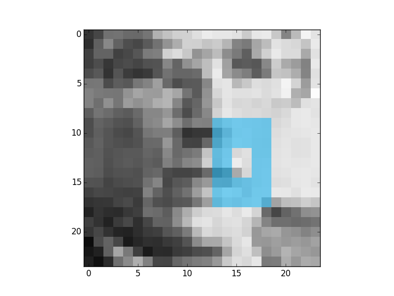
These are the first 4 most descriptive Multi-block Binary Patterns features that were found by Gentle Adaboost and binary decision trees:

And this is the first feature that was found using the same process but with the original tree from the paper:

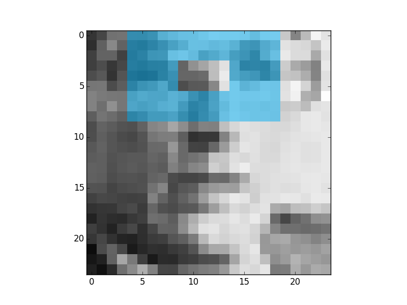
As it can be seen the result is better. Because it is more similar to the features that were derived in the Viola and Jones paper. In this case this feature says that the regions or eyes are usually darker than the regions of nose. This is an example of weak classifier. The results are like this because the binary tree is a worse classifier than a tree with 256 branches.

This is why there is still a place to improve the classifier by using trees from the paper.

Attentional Cascade.

During the implementation I stricly followed the Viola and Jones paper.

Results of the work by the end of the deadline of GSOC

By the end of the GSOC I was able to implement the efficient evaluation part for face detection. So the script uses the trained xml file from OpenCV and is able to detect faces on the image. This was made with the help of OpenMP because some parts can be done in parallel and otherwise the detection takes too long.

The training part was partially implemented and the delay was caused by the absence of information about the efficient algorithm for splitting the binary tree in case of categorical variables.