Image Classification and Segmentation with Tensorflow and TF-Slim
A post showing how to perform Image Classification and Image Segmentation with a recently released TF-Slim library and pretrained models.
Inroduction
In this post I want to show an example of application of Tensorflow and a recently released library slim for Image Classification, Image Annotation and Segmentation. In the post I focus on slim, cover a small theoretical part and show possible applications.
I have tried other libraries before like Caffe, Matconvnet, Theano and Torch. All of them have their pros and cons, but I always wanted a library in Python that is flexible, has good support and has a lot of pretrained models. Recently, a new library called slim was released along with a set of standart pretrained models like ResNet, VGG, Inception-ResNet-v2 (new winner of ILSVRC) and others. This library along with models are supported by Google, which makes it even better. There was a need for a library like this because Tensorflow itself is a very low-level and any implementation can become highly complicated. It requires writing a lot of boilerplate code. Reading other people’s code was also complicated. slim is a very clean and lightweight wrapper around Tensorflow with pretrained models.
This post assumes a prior knowledge of Tensorflow and Convolutional Neural Networks. Tensorflow has a nice tutorials on both of these. You can find them here.
The blog post is created using jupyter notebook. After each chunk of a code you can see the result of its evaluation. You can also get the notebook file from here. The content of the blog post is partially borrowed from slim walkthough notebook.
Setup
To be able to run the code, you will need to have Tensorflow installed. I have used r0.11. You will need to have tensorflow/models repository cloned. To clone it, simply run:
git clone https://github.com/tensorflow/modelsI am also using scikit-image library and numpy for this tutorial plus other dependencies. One of the ways to install them is to download Anaconda software package for python.
First, we specify tensorflow to use the first GPU only. Be careful, by default it will use all available memory. Second, we need to add the cloned repository to the path, so that python is able to see it.
import sys
import os

os.environ["CUDA_VISIBLE_DEVICES"] = '0'
sys.path.append("/home/dpakhom1/workspace/models/slim")
Now, let’s download the VGG-16 model which we will use for classification of images and segmentation. You can also use networks that will consume less memory(for example, AlexNet). For more models look here.
from datasets import dataset_utils
import tensorflow as tf

url = "http://download.tensorflow.org/models/vgg_16_2016_08_28.tar.gz"

# Specify where you want to download the model to
checkpoints_dir = '/home/dpakhom1/checkpoints'

if not tf.gfile.Exists(checkpoints_dir):
    tf.gfile.MakeDirs(checkpoints_dir)

dataset_utils.download_and_uncompress_tarball(url, checkpoints_dir)
>> Downloading vgg_16_2016_08_28.tar.gz 100.0%
Successfully downloaded vgg_16_2016_08_28.tar.gz 513324920 bytes.
Image Classification
The model that we have just downloaded was trained to be able to classify images into 1000 classes. The set of classes is very diverse. In our blog post we will use the pretrained model to classify, annotate and segment images into these 1000 classes.
Below you can see an example of Image Classification. We preprocess the input image by resizing it while preserving the aspect ratio and crop the central part. The size of the crop is equal to the size of images that the network was trained on.
%matplotlib inline
from matplotlib import pyplot as plt
import numpy as np
import os
import tensorflow as tf
import urllib2
from datasets import imagenet
from nets import vgg
from preprocessing import vgg_preprocessing
checkpoints_dir = '/home/dpakhom1/checkpoints'
slim = tf.contrib.slim
# We need default size of image for a particular network.
# The network was trained on images of that size -- so we
# resize input image later in the code.
image_size = vgg.vgg_16.default_image_size
with tf.Graph().as_default():
url = ("https://upload.wikimedia.org/wikipedia/commons/d/d9/"
"First_Student_IC_school_bus_202076.jpg")
# Open specified url and load image as a string
image_string = urllib2.urlopen(url).read()
# Decode string into matrix with intensity values
image = tf.image.decode_jpeg(image_string, channels=3)
# Resize the input image, preserving the aspect ratio
# and make a central crop of the resulted image.
# The crop will be of the size of the default image size of
# the network.
processed_image = vgg_preprocessing.preprocess_image(image,
image_size,
image_size,
is_training=False)
# Networks accept images in batches.
# The first dimension usually represents the batch size.
# In our case the batch size is one.
processed_images = tf.expand_dims(processed_image, 0)
# Create the model, use the default arg scope to configure
# the batch norm parameters. arg_scope is a very conveniet
# feature of slim library -- you can define default
# parameters for layers -- like stride, padding etc.
with slim.arg_scope(vgg.vgg_arg_scope()):
logits, _ = vgg.vgg_16(processed_images,
num_classes=1000,
is_training=False)
# In order to get probabilities we apply softmax on the output.
probabilities = tf.nn.softmax(logits)
# Create a function that reads the network weights
# from the checkpoint file that you downloaded.
# We will run it in session later.
init_fn = slim.assign_from_checkpoint_fn(
os.path.join(checkpoints_dir, 'vgg_16.ckpt'),
slim.get_model_variables('vgg_16'))
with tf.Session() as sess:
# Load weights
init_fn(sess)
# We want to get predictions, image as numpy matrix
# and resized and cropped piece that is actually
# being fed to the network.
np_image, network_input, probabilities = sess.run([image,
processed_image,
probabilities])
probabilities = probabilities[0, 0:]
sorted_inds = [i[0] for i in sorted(enumerate(-probabilities),
key=lambda x:x[1])]
# Show the downloaded image
plt.figure()
plt.imshow(np_image.astype(np.uint8))
plt.suptitle("Downloaded image", fontsize=14, fontweight='bold')
plt.axis('off')
plt.show()
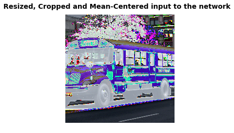
# Show the image that is actually being fed to the network
# The image was resized while preserving aspect ratio and then
# cropped. After that, the mean pixel value was subtracted from
# each pixel of that crop. We normalize the image to be between [-1, 1]
# to show the image.
plt.imshow( network_input / (network_input.max() - network_input.min()) )
plt.suptitle("Resized, Cropped and Mean-Centered input to network",
fontsize=14, fontweight='bold')
plt.axis('off')
plt.show()
names = imagenet.create_readable_names_for_imagenet_labels()
for i in range(5):
index = sorted_inds[i]
# Now we print the top-5 predictions that the network gives us with
# corresponding probabilities. Pay attention that the index with
# class names is shifted by 1 -- this is because some networks
# were trained on 1000 classes and others on 1001. VGG-16 was trained
# on 1000 classes.
print('Probability %0.2f => [%s]' % (probabilities[index], names[index+1]))
res = slim.get_model_variables()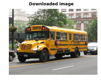
Probability 1.00 => [school bus]
Probability 0.00 => [minibus]
Probability 0.00 => [passenger car, coach, carriage]
Probability 0.00 => [trolleybus, trolley coach, trackless trolley]
Probability 0.00 => [cab, hack, taxi, taxicab]
Image Annotation and Segmentation
As you can see from the previous example, only a certain part of the original image is being processed by the network. This is good only for cases when we want to get a single prediction for an image.
Sometimes we want to get more information from an image. For example, it would be great to know about all the objects that are present in the image. For example, network would tell us that it found a school bus, other cars and building. Using this information, we can create a search engine that will be able to give us all images that has a particular object in them. This can be seen as a simple case of Image Annotation.
But what if we also want to get spatial information about the objects locations. Can the network tell us that it sees a bus in the center of the image and building on the top-right corner? That way we can create a more specific queries for a search engine: “Give me all images where the school bus is located in the middle AND flower pot in the top left corner”.
There are cases when we need to classify each pixel of the image, also know as the task of Segmentation. Imagine, that we have a huge dataset with pictures and we want to blur faces of people there, so that we don’t have to get their permission to publish these pictures. For example, you can see people’s faces being blured in Google Street View. But we only need to blur faces and not other content that might be important. Segmentation can help us in this case. We can get pixels that belong to faces and blur only them.
Below we will see a simple example of Segmentation. For the simplicity, the segmentation will be of a smaller size than the original image. We can do segmentation using an existing Convolutional Neural Network by applying it in a Fully Convolutional manner. This is done by casting the Fully Connected Layers of a network into Convolutional – this way we can input image of any size and get segmentation of lower resolution due to max-pooling layers that are used in network. To get the Segmentation of the same size as an input, deconvolutional layers can be used. You can read more about this in the paper fully convolutional networks for semantic segmentation by Long et al. We won’t consider deconvolutional layers in this example. Example below shows how to get segmentation of lower resolution than the input. Deconvolutional layers can be seen as a way to perform interpolation. Interpolation can be different (quadratic, qubic and other) but network can learn a specific interpolation that performs well under a certain task.
from preprocessing import vgg_preprocessing

# Load the mean pixel values and the function
# that performs the subtraction
from preprocessing.vgg_preprocessing import (_mean_image_subtraction,
                                            _R_MEAN, _G_MEAN, _B_MEAN)

# Function to nicely print segmentation results with
# colorbar showing class names
def discrete_matshow(data, labels_names=[], title=""):
    #get discrete colormap
    cmap = plt.get_cmap('Paired', np.max(data)-np.min(data)+1)
    # set limits .5 outside true range
    mat = plt.matshow(data,
                      cmap=cmap,
                      vmin = np.min(data)-.5,
                      vmax = np.max(data)+.5)
    #tell the colorbar to tick at integers
    cax = plt.colorbar(mat,
                       ticks=np.arange(np.min(data),np.max(data)+1))

    # The names to be printed aside the colorbar
    if labels_names:
        cax.ax.set_yticklabels(labels_names)

    if title:
        plt.suptitle(title, fontsize=14, fontweight='bold')


with tf.Graph().as_default():

    url = ("https://upload.wikimedia.org/wikipedia/commons/d/d9/"
           "First_Student_IC_school_bus_202076.jpg")

    image_string = urllib2.urlopen(url).read()
    image = tf.image.decode_jpeg(image_string, channels=3)

    # Convert image to float32 before subtracting the
    # mean pixel value
    image_float = tf.to_float(image, name='ToFloat')

    # Subtract the mean pixel value from each pixel
    processed_image = _mean_image_subtraction(image_float,
                                              [_R_MEAN, _G_MEAN, _B_MEAN])

    input_image = tf.expand_dims(processed_image, 0)

    with slim.arg_scope(vgg.vgg_arg_scope()):

        # spatial_squeeze option enables to use network in a fully
        # convolutional manner
        logits, _ = vgg.vgg_16(input_image,
                               num_classes=1000,
                               is_training=False,
                               spatial_squeeze=False)

    # For each pixel we get predictions for each class
    # out of 1000. We need to pick the one with the highest
    # probability. To be more precise, these are not probabilities,
    # because we didn't apply softmax. But if we pick a class
    # with the highest value it will be equivalent to picking
    # the highest value after applying softmax
    pred = tf.argmax(logits, dimension=3)

    init_fn = slim.assign_from_checkpoint_fn(
        os.path.join(checkpoints_dir, 'vgg_16.ckpt'),
        slim.get_model_variables('vgg_16'))

    with tf.Session() as sess:
        init_fn(sess)
        segmentation, np_image = sess.run([pred, image])

# Remove the first empty dimension
segmentation = np.squeeze(segmentation)

# Let's get unique predicted classes (from 0 to 1000) and
# relable the original predictions so that classes are
# numerated starting from zero
unique_classes, relabeled_image = np.unique(segmentation,
                                            return_inverse=True)

segmentation_size = segmentation.shape

relabeled_image = relabeled_image.reshape(segmentation_size)

labels_names = []

for index, current_class_number in enumerate(unique_classes):

    labels_names.append(str(index) + ' ' + names[current_class_number+1])

discrete_matshow(data=relabeled_image, labels_names=labels_names, title="Segmentation")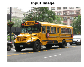
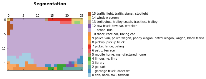
The segmentation that was obtained shows that network was able to find the school bus, traffic sign in the left-top corner that can’t be clearly seen in the image. It was able to locate windows at the top-left corner and even made a hypothesis that it is a library (we don’t know if that is true). It also made a certain number of not so correct predictions. Those are usually caused by the fact that the network can only see a part of image when it is centered at a pixel. The characteristic of a network that represents it is called receptive field. Receptive field of the network that we use in this blog is 404 pixels. So when network can only see a part of the school bus, it confuses it with taxi or pickup truck. You can see that in the bottom-left corner of segmentation results.
As we can see above, we got a simple segmentation for our image. It is not very precise because the network was originally trained to perform classification and not segmentation. If we want to get better results, we will have to train it ourselves. Anyways, the results that we got are suitable for image annotation and very approximate segmentation.
Performing Segmentation using Convolutional Neural Networks can be seen as performing classification at different parts of an input image. We center network at a particular pixel, make prediction and assign label to that pixel. This way we add spatial information to our classification and get segmentation.
Conclusion and Discussion
In this blog post we covered slim library by performing Image Classification and Segmentation. The post also explains a certain amount of theory behind both tasks.
In my opinion, slim along with pretrained models can be a very powerful tool while remaining very flexible and you can always intermix Tensorflow with it. It is relatively new, therefore, it lacks documentation and sometimes you have to read the source code. It has support from Google and is currently in an active development.